Machine Learning for Stock Trading, Part 2: Data Processing
A framework for exploratory data analysis, feature engineering, and target variable creation.
Introduction
In this series, I will break down complex Machine Learning (ML) and artificial intelligence (AI) topics in a way that anyone can understand. If you are either 1) interested in applying machine learning techniques to stock trading, or 2) considering investing in a quantitative fund/strategy/manager and want to learn more about machine learning, then this series is a great starting point. This series will be based on Python since I use it for all my machine learning code. Note that this series is meant to be used as a framework/checklist for your machine learning project, and I will not be doing a deep dive on technical concepts and skills. I encourage you to perform additional research as you encounter subjects where you need a deeper understanding.
In Part 1, I laid out a high-level framework for acquiring financial time series data. If you haven’t read it yet, check it out here. In this piece, I will go over exploratory data analysis, feature engineering, and output creation.
Data is the most important aspect of any machine learning project. There is a common saying in machine learning: “Garbage in, garbage out.” In other words, it doesn’t matter how good a model is, its results will only be as good as the underlying data. That’s why it’s extremely important to spend extra time in the beginning to get the data right.
1. Reading Data with Pandas
Once you’ve acquired your data, you are ready to start working with it in pandas. As discussed in Part 1, I highly recommend using pandas to work with data in Python. The data object that is used by pandas is called a DataFrame. You can think of a DataFrame as a more versatile version of an Excel spreadsheet.
Most financial data will be delivered as CSV, Excel, or JSON files. You can use pandas builtin functions read_csv, read_excel, and read_json, respectively, to convert your data into DataFrame form. Some data already comes in DataFrame form, which makes things really easy.
2. Exploratory Data Analysis
Once you have your data in a DataFrame, you are ready to perform exploratory data analysis (EDA). EDA is a standard and crucial step in all data science related projects. It is the process of investigating your data to discover patterns and spot anomalies. For EDA, most machine learning researchers will use Python libraries matplotlib and seaborn.
2.2 Summary Statistics
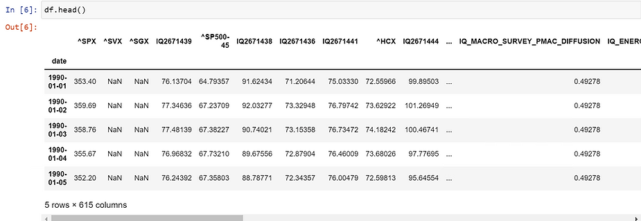
The first step of EDA is to examine your DataFrame at a high level. Use pandas head, tail, and describe functions to do this. The head and tail functions output the first and last 5 lines of your DataFrame. The describe function outputs summary statistics. Pay close attention to the mean, standard deviation, and min/max values as they will help you in items 3-5 below.
Head Function

Describe Function
2.3 Data Visualization
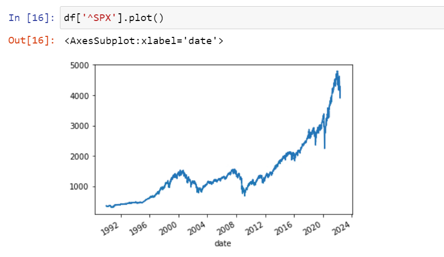
Next, it’s time to visualize your data. For trended financial time series data, you can use matplotlib’s plot function to visualize the trend. You will ultimately want to detrend trended time series data (more on that in item 5 below).

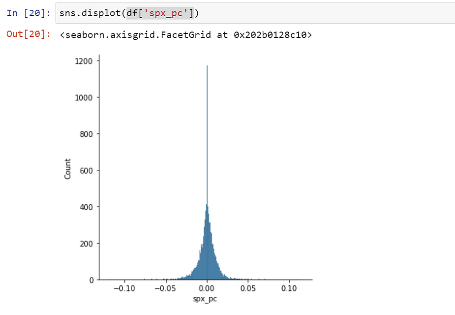
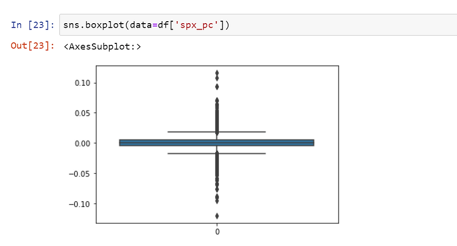
For detrended time series data, use seaborn’s distplot in conjunction with boxplot to visualize the distribution and identify outliers.
Distplot
Boxplot
If you are working with categorical data, you can use seaborn’s countplot function to visualize the distribution.
These are just some of the standard functions you can use to explore your data. Other functions may be more suited to your project. Whatever you end up using, the most important thing is to understand what your data looks like so that you can properly address data anomalies and engineer effective features (discussed below).
3. Dealing with Missing Values
3.1 NaNs
Missing values are an important problem to address in any machine learning project. Missing values are denoted as NaN (not a number) in Python and often represented with numpy.nan (NumPy is the standard scientific computing library in Python).
NaNs occur when data is missing or corrupted. You can analyze NaNs in your DataFrame with the pandas isna function. So what is the best way to deal with NaNs? There are three main methods: Filling, imputing, and replacing with zero. The best method depends on your specific dataset.
3.2 Filling Missing Values
Filling is the process of replacing NaNs with the last known value in a data series and is best suited for continuous time series data. For example, say you are working with stock price data, and your dataset includes both weekdays and weekends. Since stocks only trade on weekdays, your data will contain NaNs on the weekends. You could address this issue by forward filling Friday’s stock price to Saturday and Sunday. Filling can be done on both a forward and backward basis using pandas ffill and bfill functions, respectively.
3.3 Imputing Missing Values
Imputing is the process of replacing NaNs with the mean or median of a data series and is best suited for detrended data (more on detrending in item 5 below). For example, say you are working with the percent change of a stock’s price and are missing some data. In this case, it would not make sense to fill missing data because that would likely skew the series. One possible solution is to replace missing values with the mean or median of the entire series. This way, you would avoid skewing the data.
3.4 Replacing Missing Values
Replacing NaNs with zero can be done on any type of data so long as you believe the data was truly missing. For example, say you are working with a fundamental dataset that contains multiple companies, and one of the features is gross margin. Not every company will have gross margin as a line item. In this case, filling or imputing missing gross margin values would have disastrous effects on your dataset. Instead, you should use the pandas fillna function to replace NaNs with zero.
4. Dealing with Outliers
4.1 What are Outliers?
Outliers are samples in the dataset that fall outside the overall pattern of the distribution. They are extremely important to address because machine learning algorithms are very sensitive to the range and distribution of the dataset. Unaddressed outliers can reduce model accuracy and increase training time.
4.2 Outlier Detection
It’s important to note that there isn’t one standard method to define outliers. The method you choose, if any, will depend on your specific dataset, project, and discretion. For example, you may decide that you do not want to address potential outliers because they could be relevant to the problem you are trying to solve. However, let’s assume that you do want to deal with outliers. I will go over three popular methods for detecting outliers and two popular methods for addressing outliers.
4.2.1 Outlier Visualization
The first method for outlier detection is visualization, which we went over in item 2. You can plot the distribution of the data using a histogram or box plot and manually select upper and lower bounds. Any datapoint falling outside of the upper and lower bounds can be considered an outlier.
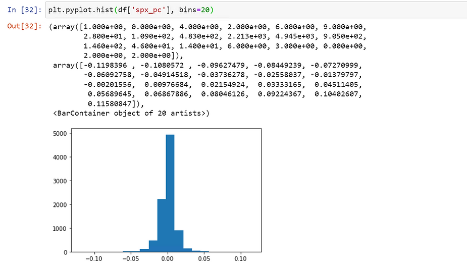
This method works well for small datasets, but is too time consuming for datasets with large numbers of features. For large datasets, try methods two or three below.
4.2.2 Extreme Value Analysis
The second method for outlier detection is called extreme value analysis. First, calculate the 1st and 3rd quartiles (Q1 and Q3). Next, calculate the interquartile range (IQR), where IQR = Q3 - Q1. Next, set upper and lower bounds for your data series. Typically, upper bound = Q3 + (IQR * 1.5) and lower bound = Q1 - (IQR * 1.5). For extreme cases, you could increase the factor from 1.5 to 3, so upper bound = Q3 + (IQR * 3) and lower bound = Q1 - (IQR * 3). Any datapoint that falls above the upper bound or below the lower bound can be considered an outlier.
4.2.3 Z-Score Analysis
The third method for outlier detection is the Z-score method. In statistics, the Z-score represents how many standard deviations a given sample is from the mean. The Z-score is calculated as: Z-score = (x - mean) / standard deviation, where x is the sample in question. Typically, samples with a Z-score >= 3 or <= -3 can be considered outliers.
4.3 Addressing Outliers
Once you’ve determined which samples are outliers, select a way to address them. Two of the most popular methods are replacing and trimming. The method you use will again be specific to your dataset and project.
4.3.1 Replacing Outliers
Replacing outliers: If you believe that the outliers are genuine data points (i.e. not the result of error), then you could replace them with the mean or median of the data series. You could also replace the outliers with randomly sampled observations from your data series. For genuine data points, I will reiterate that you may or may not decide to address outliers based on the specific problem you are trying to solve.
4.3.2 Trimming Outliers
Trimming outliers: On the other hand, if you believe that the outliers are the result of error, then you could simply remove those observations from your data series.
5. Feature Engineering
Now that you have explored and cleaned your dataset, it’s time to move ahead with feature engineering. For financial time series data, there are two main aspects to feature engineering: Detrending time series data and new feature creation.
5.1 Detrending Time Series Data
The first thing you should do is to detrend all time series data. Trended time series data shows the movement of a series to higher or lower values over a period of time. In other words, the distribution of trended data changes over time. Remember that machine learning algorithms are highly sensitive to the distribution of the data, which is why you should always detrend time series data. The two main ways of detrending data are to take the percent changes between observations or to take the differences between observations. For financial time series data, percent changes are most often used.
Imagine you are working with the stock price of AAPL. In 2019, AAPL’s price was in the $40s; in 2020, it was in the $70s; and in 2021, it was in the $100s. In this case, the general trend of the data is upward. However, the values of the stock prices will not provide machine learning models with any meaningful information as the distribution is changing year to year.
For example, consider two cases: 1) AAPL’s stock price increases 1% from $100 to $101, and 2) AAPL’s stock price increases 2% from $50 to $51. Case 2 should result in a larger signal, however there is no way for a model to understand this. Instead, a model will think that case 1 is more meaningful since $100 is greater in value than $50.
Instead, detrend the data by calculating the percent change in stock price. Now, we have a data series that has a consistent distribution across all years. Back to our two cases: Case 1 will now have a percent change of 1% and case 2 a percent change of 2%. Now, a model can properly learn that case 2 is more meaningful than case 1.

Trended Data
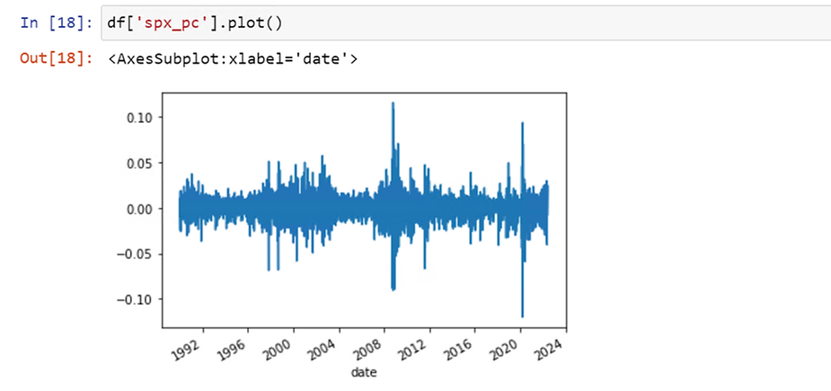
Detrended data
5.2 New Feature Creation
After detrending data, the next step is to create new features. New features consist of any feature that is created from the original dataset. Create features that are relevant for your specific dataset and project. For example, if you are working with technical data, you might want to create features such as moving averages, RSI, and Bollinger Bands. If you are working with fundamental data, you might want to calculate metrics like revenue growth, EBITDA margin, quick ratio, and P/E. If you are working with macroeconomic data, you might want to calculate items such as Treasury yield curves and the change in the Federal Funds rate.
Once you have completed the feature engineering process, it’s always a good idea to go back and through items 2-4 (exploratory data analysis, dealing with missing values, and dealing with outliers) with your new features.
6. Dimensionality Reduction
6.1 Curse of Dimensionality
In machine learning, the curse of dimensionality indicates that modeling a dataset becomes exponentially more difficult with each additional input feature. Specifically, as the number of features increases, the data becomes more sparse (i.e. it becomes harder to group the data due to the large number of dimensions). When data is sparse, machine learning algorithms tend to overfit the data, which is what we want to avoid. So in order to avoid overfitting, the number of samples in the data must be significantly increased. This is a problem because such samples may not exist; and even if they do exist, the computing power and training time needed to process such a large dataset may not be feasible.
As recent advances in computing power have enabled machine learning algorithms to handle more and more features, it may be tempting to throw the whole kitchen sink at your model. However, this is not best practice as we want to ultimately avoid the curse of dimensionality, which is why dimensionality reduction is an important step. Dimensionality reduction is the process of reducing the feature space of a dataset by removing weakly correlated features. Weakly correlated features introduce noise to machine learning algorithms and lead to longer training times and suboptimal results. I will go over three popular ways to approach dimensionality reduction. Note that many other methods exist, and I encourage you to perform additional research as necessary.
6.2 Feature Selection
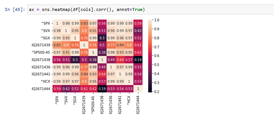
The first method for dimensionality reduction is manually selecting features for inclusion/removal. Seaborn’s heatmap function is great for visualizing the intercorrelation between features. Other popular correlation coefficients include Pearson’s Correlation Coefficient, Pearson’s Rank Correlation, and Spearman rank order correlation. Simply calculate the intercorrelation of features and remove features that fall below some lower bound (e.g. you might decide to remove features with a correlation of less than 0.5).
6.3 Principal Component Analysis
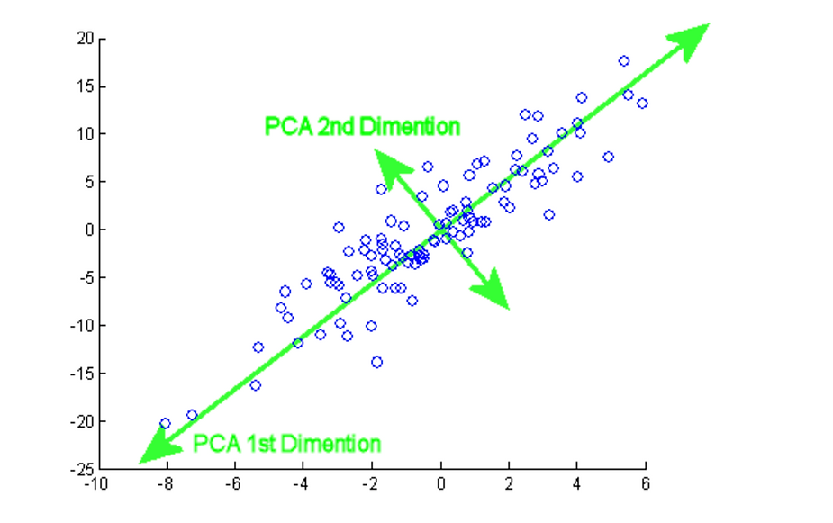
Principal Component Analysis (PCA) is commonly used to reduce the dimensionality of continuous data. I will not go into detail here, but the idea is that PCA reduces the number of features by projecting them onto a lower dimensional space. The old feature set is replaced by a smaller number of principal components, which can be used as inputs in machine learning models. You can use sci-kit learn’s PCA function to perform PCA on your data.
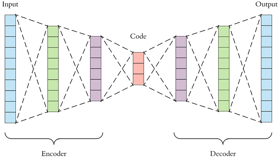
6.4 Autoencoders
An autoencoder is a type of artificial neural network that aims to copy its inputs to its outputs. Imagine a neural network with an encoder and a decoder. The encoder compresses all features into a latent-space (i.e. lower dimensional) representation. The decoder reconstructs the features from the latent-space representation. The lower dimensional representation of the data that is created by the autoencoder can be used as the input to machine learning models.
6.5 Permutation Feature Importance
Permutation feature importance is the process of calculating how important each feature is to a model by iteratively breaking the relationship between each feature and the target. For example, let’s say you want to train a complex deep learning model, for which computation power and time will be expensive. Before training the full model, you would like to remove unnecessary features so as to optimize the training process. First, train a simple model on your dataset and calculate a model score (e.g. accuracy, precision, recall, F1, etc.) on the test set. Then, pick one feature and randomly permute it, thereby breaking its relationship with the target. Next, test the model on the permuted dataset and record the score. The score will obviously change since one of the features has been permuted. Do this for each feature in the dataset. The features that resulted in the largest decreases in model score are the most important features. Some features will result in smaller decreases, or even increases, in the model score – those are the least important features and can be removed.
7. Data Standardization
7.1 What is Data Standardization?
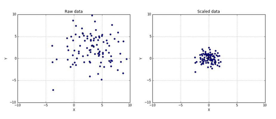
Data standardization is the process of transforming the data such that the mean of the observed values is 0 and the standard deviation is 1. The goal of standardization is to rescale all features to a common scale without distorting the differences in the range of values. Because machine learning models are very sensitive to the distribution of the data, standardized datasets will result in faster training times and better results.
7.2 Why is Standardization Important?
For example, imagine a dataset with two features: percent change in stock price and P/E ratio. P/E ratios typically have larger values than percent changes. As of the time of writing, the average P/E ratio of the S&P 500 is around 30, whereas the average daily percent change in the S&P 500 is between -0.01 and 0.01. As you can see, there is a significant scale and distribution discrepancy between the two features. If the two features were used as inputs to a machine learning model, the model would incorrectly assign more importance to the P/E ratio due to its larger scale. In order to avoid this, we standardize each feature such that both features have a mean of 0 and standard deviation of 1. Once both features are on the same scale and distribution, our machine learning model can function properly.
7.3 Using Sci-Kit Learn to Standardize Data
To standardize your data, you can use sci-kit learn’s Standard Scaler or MinMax Scaler functions.
8. Target Variable Creation
8.1 What is a Target Variable?
The final step of data processing is to create the target variable. The target variable is the dependent variable that we are trying to model. For example, assume we are using historical stock price data to model the future 1-day change in stock price. All of the features derived from historical stock price data are the inputs to our model. The target variable, or model output, is the future 1-day change in stock price.
8.2 Supervised vs Unsupervised Algorithms
In machine learning, there are two main buckets of algorithms: supervised and unsupervised. Before we continue with target variable creation, it’s important to note the difference between the two. Unsupervised algorithms learn patterns from unlabeled data. In other words, unsupervised algorithms do not have a target variable. For example, PCA (from item 6) is a type of unsupervised algorithm. On the other hand, supervised algorithms model data by mapping inputs to outputs and, therefore, do have target variables. In our example above, the future 1-day change in stock price would be our target variable. For the purposes of this series, I will assume you are working with supervised algorithms.
8.3 Continuous Variables
A continuous variable is defined as a variable which can take on an infinite set of values. If you decide you want to create an algorithm to predict a continuous variable, then you would create the target variable and use a regression-based algorithm to model your data (more on this in part 3 of this series).
Going back to our previous example, the future 1-day change in stock price is a continuous variable. Calculate the percent change of your stock price data, then organize it in an array with time on the y-axis and the percent change on the x-axis. Use this array as the target variable of a regression model.
8.4 Categorical Variables
A discrete variable, in contrast to a continuous variable, is defined as a variable that can take on one of a fixed number of possible values. For example, let’s say we want to predict whether the future 1-day change in stock price is either positive or negative. In this case, the target variable is categorical with two classes. To create these labels, you would take the future 1-day change in stock price and assign them a class based on their values: 0 if x < 0 and 1 if x >= 1, where x is the future 1-day change in stock price. Again, you would organize this data in an array with time on the y-axis and the labels on the x-axis.
Now, let’s say we want to predict whether the future 1-day change in stock price is either positive, negative, or flat. In this case, we also have a categorical target variable with three classes. To create these labels, assign 0 if x < 0, 1 if x = 0, and 2 if x > 0, where x is the future 1-day change in stock price.
In machine learning, binary classification algorithms are used to model target variables with two classes (0 or 1), and multivariate classification algorithms are used to model target variables with multiple classes (0, 1, 2, 3, and so on). Again, more on these types of models will be discussed in part 3 of this series.
8.5 Multiple Target Variables
Some machine learning algorithms also have the ability to predict multiple target variables. For example, a model could be trained to predict the future 1, 2, and 3 day change in stock price. Similarly, a model could also be trained to classify whether the future 1, 2, and 3 day changes in stock prices are positive or negative. This data is also organized as an array with time on the y-axis and multiple target variables on the x-axis.
Final Thoughts
Once you have processed your data, it’s time to create and train your machine learning algorithms. In the next piece, I will cover model architecture and training/evaluating machine learning models.
What about alphaAI?
In any investment endeavor, the key to success lies in making informed decisions. Whether you're building a recession-resistant portfolio, diversifying your assets, or simply exploring new opportunities, your journey should be guided by knowledge and insight. At alphaAI, we are dedicated to helping you invest intelligently with AI-powered strategies. Our roboadvisor adapts to market shifts, offering dynamic wealth management tailored to your risk level and portfolio preferences. We're your trusted partner in the complex world of finance, working with you to make smarter investments and pursue your financial goals with confidence. Your journey to financial success begins here, with alphaAI by your side.
Supercharge your trading strategy with alphaAI.
Discover the power of AI-driven trading algorithms and take your investments to the next level.

Explore Our Blog
Stay updated with our latest blog posts.

The Power of the Magnificent 7 and How alphaAI Uses FNGU to Make It Accessible

Politician Stock Tracker Insights: The Allure of Congress Stock Trades and Nancy Pelosi’s Portfolio


